Plotting Examples

One of the core features of HPMOC is its robust and convenient suite of plotting tools. This page includes several examples showcasing how to use HPMOC for sophisticated plots. An emphasis is made on showing how to navigate different tools and projections, and how to quickly iterate to get a perfect plot for your purposes.

HPMOC uses the astropy.wcs.WCS implementation of FITS projections for plotting. Details of the projection definitions and their associated FITS header keywords are given in Calabretta and Greisen (2002).

Setup

We’ll start by importing packages and picking some skymap files of various types from the test skymaps included in the HPMOC source repository. The loading and plotting instructions in this document work with any skymaps produced by any of the major LIGO pipelines (in particular, anything downloaded from GraceDB should work).

[1]:

from pathlib import Path
import numpy as np
from matplotlib import pyplot as plt
from hpmoc import PartialUniqSkymap
from hpmoc.plot import get_wcs, plot, gridplot

DATA = Path(".").absolute().parent.parent.parent/"tests"/"data"

NUNIQ_FITS = DATA/'S200105ae.fits'
NUNIQ_FITS_GZ = DATA/'S200105ae.fits.gz'
BAYESTAR_NEST_FITS_GZ_1024 = DATA/'S200316bj-1-Preliminary.fits.gz'
CWB_NEST_FITS_GZ_128 = DATA/'S200114f-3-Initial.fits.gz'
CWB_RING_FITS_GZ_128 = DATA/'S200129m-3-Initial.fits.gz'

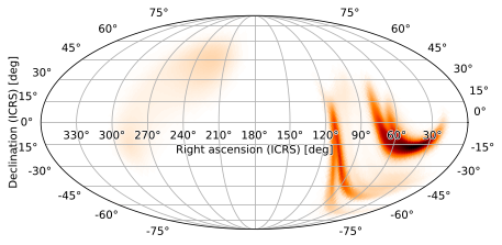
Basic Plotting

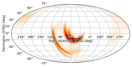
We can easily load and display a skymap using the default plot settings, which produce a Mollweide plot, using hpmoc.partial.PartialUniqSkymap.plot (a thin wrapper around hpmoc.plot.plot):

[2]:

m = PartialUniqSkymap.read(NUNIQ_FITS, strategy='ligo')
# Replace the above line with the following (the GraceDB URL of the same skymap)
# if you don't have the test files handy:
# m = PartialUniqSkymap.read(graceid, 'bayestar.multiorder.fits,0',
#                            strategy='gracedb')
m.plot()

[2]:

<astropy.visualization.wcsaxes.core.WCSAxes at 0x11a40df90>

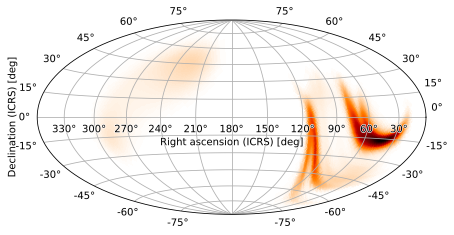
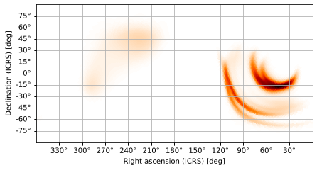
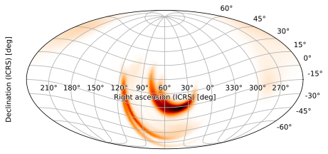
../_images/jup_plotting-examples_3_1.png

We can modify various properties; for example, we can double the default pixel height (vertical resolution) of the rendered image by doubling the height; the pixel width will not change, and so the aspect ratio will change:

[3]:

m.plot(height=360)

[3]:

<astropy.visualization.wcsaxes.core.WCSAxes at 0x121034590>

../_images/jup_plotting-examples_5_1.png

We can also change the size of the figure itself, either by creating a new matplotlib.figure.Figure and passing it as the fig argument, or by simply passing the same keywords we would use for Figure as the fig argument to plot:

[4]:

m.plot(fig={'figsize': (12, 8)}, height=360, width=720)

[4]:

<astropy.visualization.wcsaxes.core.WCSAxes at 0x1206c1910>

../_images/jup_plotting-examples_7_1.png

We can also add color bars with the cbar argument:

[5]:

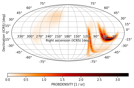
m.plot(cbar=True)

[5]:

<astropy.visualization.wcsaxes.core.WCSAxes at 0x1208c4c90>

../_images/jup_plotting-examples_9_1.png

We can plot all-sky fixed HEALPix order skymaps with implicit pixel indices by passing the data arrays to plot as well. We can do this by instantiating a PartialUniqSkymap using the pixels and ordering:

[6]:

from astropy.table import Table

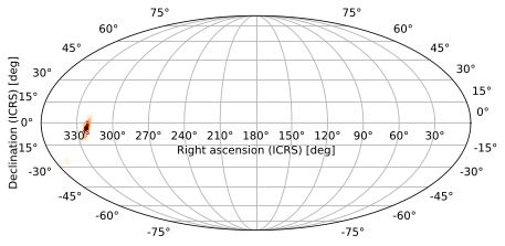
t1 = Table.read(CWB_RING_FITS_GZ_128)
PartialUniqSkymap(t1['PROB'].ravel(), t1.meta['ORDERING']).compress().plot()

[6]:

<astropy.visualization.wcsaxes.core.WCSAxes at 0x12589ab10>

../_images/jup_plotting-examples_11_1.png

or by passing the arguments as a tuple to hpmoc.plot.plot, which does the same thing behind the scenes for us:

[7]:

t2 = Table.read(CWB_NEST_FITS_GZ_128)
plot((t2['PROB'].ravel(), t2.meta['ORDERING']))

[7]:

<astropy.visualization.wcsaxes.core.WCSAxes at 0x120e17790>

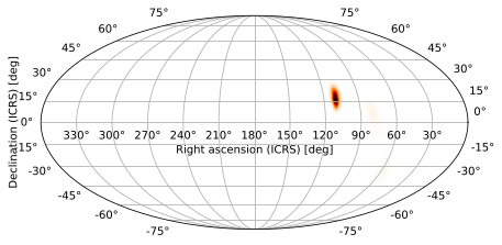
../_images/jup_plotting-examples_13_1.png

As you can see, this worked on both a RING-ordered and a NESTED-ordered skymap:

[8]:

print(t1.meta['ORDERING'], t2.meta['ORDERING'])

RING NESTED

One advantage of loading into PartialUniqSkymap first is that we can call the compress method to eliminate redundant pixels first. This will not have a tremendous effect if we are doing a one-off plot, but it can lead to multiple orders of magnitude of performance increase (particularly with BAYESTAR skymaps) if we are going to work with the skymaps repeatedly. If you load a skymap with PartialUniqSkymap.read, as we did earlier, all of this is handled for you; the skymap is even read in small chunks to avoid ever using much of a memory footprint. It also takes care of the slight differences between LIGO pipelines’ skymap formats for you. Nonetheless, if you come across a HEALPix skymap that’s not already supported, you can still load and plot it in HPMOC.

There are many other arguments available to tweak the look and feel of the plot; see some of the specific examples below as well as the full documentation in hpmoc.plot.plot.

Projections

There are, however, many other projections available. The ones with built-in HPMOC support are discussed in this section.

Cylindrical and Pseudocylindrical projections

Mollweide Projection

The Mollweide (MOL) projection is an example of a pseudocylindrical projection. We can explicitly select the Mollweide projection by passing "Mollweide", or its FITS projection code, "MOL" (or any of the aliases specified in hpmoc.plot.get_wcs), as the projection argument to plot

[9]:

m.plot(projection='Mollview')  # same as projection='MOL'

[9]:

<astropy.visualization.wcsaxes.core.WCSAxes at 0x12751a190>

../_images/jup_plotting-examples_18_1.png

Hammer-Aitoff Projection

Other useful pseudocylindrical projections include the Hammer-Aitoff projection (AIT)

[10]:

m.plot(projection='AIT')

[10]:

<astropy.visualization.wcsaxes.core.WCSAxes at 0x12092b150>

../_images/jup_plotting-examples_20_1.png

Cylindrical equal-area

the cylindrical equal-area projection, which preserves areas

[11]:

m.plot(projection='CEA')

[11]:

<astropy.visualization.wcsaxes.core.WCSAxes at 0x127552d10>

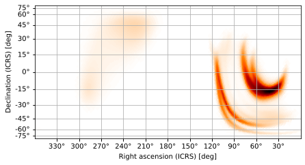
../_images/jup_plotting-examples_22_1.png

Plate Carée Projection

and the (Cylindrical) plate carée (CAR), AKA Cartesian, projection, which maps latitude and longitude coordinates one-to-one.

[12]:

m.plot(projection='CAR')

[12]:

<astropy.visualization.wcsaxes.core.WCSAxes at 0x1261a7110>

../_images/jup_plotting-examples_24_1.png

Zenithal Projections

Zenithal projections are radially symmetric in their distortion and tend to be better suited to plotting zoomed images.

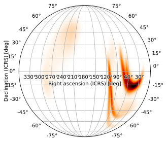
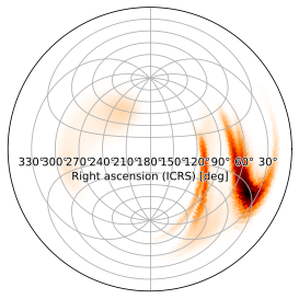
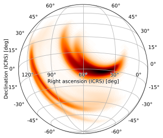
Slant Orthographic Projection

One exception is the slant orthographic (SIN) projection, which (with default settings) looks like a globe viewed from a great distance with the image plotted on its surface:

[13]:

m.plot(projection='SIN')

[13]:

<astropy.visualization.wcsaxes.core.WCSAxes at 0x126c964d0>

/Users/s/anaconda3/envs/hpmoc-dev/lib/python3.7/site-packages/astropy/visualization/wcsaxes/grid_paths.py:73: RuntimeWarning: invalid value encountered in greater
  discontinuous = step[1:] > DISCONT_FACTOR * step[:-1]
/Users/s/anaconda3/envs/hpmoc-dev/lib/python3.7/site-packages/astropy/visualization/wcsaxes/grid_paths.py:73: RuntimeWarning: invalid value encountered in greater
  discontinuous = step[1:] > DISCONT_FACTOR * step[:-1]
/Users/s/anaconda3/envs/hpmoc-dev/lib/python3.7/site-packages/astropy/visualization/wcsaxes/grid_paths.py:73: RuntimeWarning: invalid value encountered in greater
  discontinuous = step[1:] > DISCONT_FACTOR * step[:-1]
/Users/s/anaconda3/envs/hpmoc-dev/lib/python3.7/site-packages/astropy/visualization/wcsaxes/grid_paths.py:73: RuntimeWarning: invalid value encountered in greater
  discontinuous = step[1:] > DISCONT_FACTOR * step[:-1]

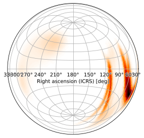
../_images/jup_plotting-examples_26_2.png

Note that WCSAxes don’t handle the tick labels well for slant orthographic projections; you will get warnings and missing or strangely-positioned tick labels, as in the plots on this page, when plotting this projection. You can fix the labels manually by playing with ax.coord, but the easiest solution is to increase the plot resolution (at the expense of plotting speed), as is done in all of the remaining SIN skymaps in this document using the height and width parameters:

[14]:

m.plot(height=720, width=720, projection='SIN')

[14]:

<astropy.visualization.wcsaxes.core.WCSAxes at 0x1268333d0>

/Users/s/anaconda3/envs/hpmoc-dev/lib/python3.7/site-packages/astropy/visualization/wcsaxes/grid_paths.py:73: RuntimeWarning: invalid value encountered in greater
  discontinuous = step[1:] > DISCONT_FACTOR * step[:-1]
/Users/s/anaconda3/envs/hpmoc-dev/lib/python3.7/site-packages/astropy/visualization/wcsaxes/grid_paths.py:73: RuntimeWarning: invalid value encountered in greater
  discontinuous = step[1:] > DISCONT_FACTOR * step[:-1]
/Users/s/anaconda3/envs/hpmoc-dev/lib/python3.7/site-packages/astropy/visualization/wcsaxes/grid_paths.py:73: RuntimeWarning: invalid value encountered in greater
  discontinuous = step[1:] > DISCONT_FACTOR * step[:-1]
/Users/s/anaconda3/envs/hpmoc-dev/lib/python3.7/site-packages/astropy/visualization/wcsaxes/grid_paths.py:73: RuntimeWarning: invalid value encountered in greater
  discontinuous = step[1:] > DISCONT_FACTOR * step[:-1]

../_images/jup_plotting-examples_28_2.png

Gnomonic Projection

The gnomonic (TAN) projection is most often uzed for zoomed views of a specific region of the sky. Its default zoom level in HPMOC is chosen to be the same as that used by healpy.gnomview.

[15]:

m.plot(projection='TAN')

[15]:

<astropy.visualization.wcsaxes.core.WCSAxes at 0x125a66d90>

../_images/jup_plotting-examples_30_1.png

Zenithal Equidistant Projection

The zenithal equidistant (ARC) projection is similarly suitable for this purpose, though by default it produces an all-sky view

[16]:

m.plot(projection='ARC')

[16]:

<astropy.visualization.wcsaxes.core.WCSAxes at 0x126990910>

../_images/jup_plotting-examples_32_1.png

Zenithal Equal-Area Projection

as does the zenithal equal-area (ZEA) projection:

[17]:

m.plot(projection='ZEA')

[17]:

<astropy.visualization.wcsaxes.core.WCSAxes at 0x125a5cf90>

../_images/jup_plotting-examples_34_1.png

Arbitrary `WCS` Projections

These are likely to be the most useful projections for most purposes. However, any valid astropy.wcs.WCS instance capable of being plotted on an astropy.visualization.wcsaxes.WCSAxes can be passed as the projection argument. This is, in fact, how hpmoc.plot.plot works behind the scenes; you can separate this step out explicitly by calling hpmoc.plot.get_wcs to construct a WCS instance

[18]:

w = get_wcs('MOL')
w

[18]:

WCS Keywords

Number of WCS axes: 2
CTYPE : 'RA---MOL'  'DEC--MOL'
CRVAL : 180.0  0.0
CRPIX : 180.5  90.5
PC1_1 PC1_2  : 1.0  0.0
PC2_1 PC2_2  : 0.0  1.0
CDELT : -0.9003163161571062  0.9003163161571062
NAXIS : 360.0  180

which can be used as the projection argument. Note that hpmoc.plot.plot will not automatically select the frame around the plot when passed a WCS instance as the projection, so we need to explicitly specify an elliptical frame:

[19]:

m.plot(projection=w, frame_class='elliptical')

[19]:

<astropy.visualization.wcsaxes.core.WCSAxes at 0x1267531d0>

../_images/jup_plotting-examples_38_1.png

Being able to use arbitrary WCS instances as the projection makes it easy to overplot HEALPix skymaps on the same axes as images from the many observatories that store data using FITS.

Regardless of how a projection is specified, a WCSAxes instance will always be returned, and its wcs field will hold the resulting projection:

[20]:

m.plot().wcs

[20]:

WCS Keywords

Number of WCS axes: 2
CTYPE : 'RA---MOL'  'DEC--MOL'
CRVAL : 180.0  0.0
CRPIX : 180.5  90.5
PC1_1 PC1_2  : 1.0  0.0
PC2_1 PC2_2  : 0.0  1.0
CDELT : -0.9003163161571062  0.9003163161571062
NAXIS : 360.0  180

../_images/jup_plotting-examples_40_1.png

Rotations

hpmoc.plot.plot puts a right ascension of 180 degrees at the center of the skymap (the default used by the LIGO collaboration for their skymaps). We can rotate the skymap to have a different center with the rot argument, which specifies the three Euler angles (rotating about the ZXZ reference axes) for rotating the skymap.

2-Angle Rotations

In practice, one usually simply wants to specify the coordinates at the center of the image. HPMOC handles this automatically for all built-in projections when provided only the right ascension and declination of the central point for the rot argument. For example, we can center a high-probability region at RA=60, dec=-15 by passing those as the rot argument:

[21]:

m.plot(rot=(60, -15))

[21]:

<astropy.visualization.wcsaxes.core.WCSAxes at 0x1267c07d0>

../_images/jup_plotting-examples_42_1.png

Again, this works for any built-in projection and is usually what you want to do. The final angle corresponding to the FITS WCS LONPOLE keyword is calculated automatically so that the rotation is well-defined and the vertical direction at the center of the image points towards the north pole.

3-Angle Rotations

Sometimes, however, this isn’t enough. You may need to specify a custom WCS for which HPMOC cannot automatically calculate LONPOLE, or you may want to apply an additional rotation to your plot. This section briefly discusses how rot is translated into FITS WCS keywords and how their interpretation varies accross different categories of projection.

The details of how rotations are set vary by projection; in particular, the valid angle combinations are not always intuitive. One can figure out the valid angles by referencing the projection definitions in Calabretta and Greisen (2002), though in practice a little bit of trial an error usually suffices to figure out the correct choices. The three components of the rot argument tuple are used directly as the CDELT1, CDELT2, LONPOLE FITS header fields (explained in that document) for specifying a WCS.

HPMOC uses these coordinate definitions, non-intuitive properties and all, in the belief that cross-compatibility (with FITS in general and ``astropy.wcs.WCS`` in particular) outweigh the slight learning curve; that the unintuitive behaviors can be quickly learned with a little bit of documentation; and that the exceptional cases where ``LONPOLE`` need be specified are too rare to justify additional code complexity.

The effect of the rot arguments is mostly within a certain category of projections; we will therefore discuss rotations in (pseudo)cylindrical and zenithal projections with separate examples.

Rotations in Cylindrical and Pseudocylindrical Projections

In this section we will consider the Mollweide projection, though the conclusions should mostly apply to the other (pseudo)cylindrical projections (Hammer-Aitoff and plate carée) as well.

We can center the skymap on a right-ascension of 60 degrees as follows:

[22]:

m.plot(rot=(60, 0, 0))

[22]:

<astropy.visualization.wcsaxes.core.WCSAxes at 0x1274b2510>

../_images/jup_plotting-examples_44_1.png

In the Mollweide projection, we can center the plot on a point with positive declination by providing it as the second angle in rot. For example, we can center the plot on RA = 60, DEC = 15 as follows:

[23]:

m.plot(rot=(60, 15, 0))

[23]:

<astropy.visualization.wcsaxes.core.WCSAxes at 0x126452690>

../_images/jup_plotting-examples_46_1.png

We will get an error if we try to set the second Euler angle to -15 degrees, however, as we might want to do in this case to center the skymap on the region of highest probability. This can be fixed by setting the final angle to 180.

[24]:

m.plot(rot=(60, -15, 180))

[24]:

<astropy.visualization.wcsaxes.core.WCSAxes at 0x1267b0ad0>

../_images/jup_plotting-examples_48_1.png

Rotations in Zenithal Projections

In this section we will consider the slant orthographic projection, though the conclusions should mostly apply to the other zenithal projections (gnomonic, zenithal equidistant, zenithal equal-area) as well.

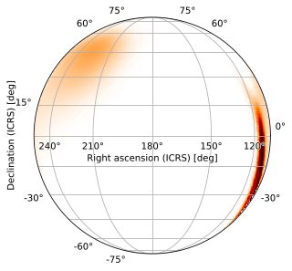
The rot argument works more straightforwardly in zenithal projections, with a caveat. We can specify any right ascension and declination, e.g. a positive declination

[25]:

m.plot(height=720, width=720, projection='SIN', rot=(60, 15, 0))

[25]:

<astropy.visualization.wcsaxes.core.WCSAxes at 0x1270fa810>

/Users/s/anaconda3/envs/hpmoc-dev/lib/python3.7/site-packages/astropy/visualization/wcsaxes/grid_paths.py:73: RuntimeWarning: invalid value encountered in greater
  discontinuous = step[1:] > DISCONT_FACTOR * step[:-1]
/Users/s/anaconda3/envs/hpmoc-dev/lib/python3.7/site-packages/astropy/visualization/wcsaxes/grid_paths.py:73: RuntimeWarning: invalid value encountered in greater
  discontinuous = step[1:] > DISCONT_FACTOR * step[:-1]
/Users/s/anaconda3/envs/hpmoc-dev/lib/python3.7/site-packages/astropy/visualization/wcsaxes/grid_paths.py:73: RuntimeWarning: invalid value encountered in greater
  discontinuous = step[1:] > DISCONT_FACTOR * step[:-1]
/Users/s/anaconda3/envs/hpmoc-dev/lib/python3.7/site-packages/astropy/visualization/wcsaxes/grid_paths.py:73: RuntimeWarning: invalid value encountered in greater
  discontinuous = step[1:] > DISCONT_FACTOR * step[:-1]

../_images/jup_plotting-examples_50_2.png

or negative one

[26]:

m.plot(height=720, width=720, projection='SIN', rot=(60, -15, 0))

[26]:

<astropy.visualization.wcsaxes.core.WCSAxes at 0x12737db90>

/Users/s/anaconda3/envs/hpmoc-dev/lib/python3.7/site-packages/astropy/visualization/wcsaxes/grid_paths.py:73: RuntimeWarning: invalid value encountered in greater
  discontinuous = step[1:] > DISCONT_FACTOR * step[:-1]
/Users/s/anaconda3/envs/hpmoc-dev/lib/python3.7/site-packages/astropy/visualization/wcsaxes/grid_paths.py:73: RuntimeWarning: invalid value encountered in greater
  discontinuous = step[1:] > DISCONT_FACTOR * step[:-1]
/Users/s/anaconda3/envs/hpmoc-dev/lib/python3.7/site-packages/astropy/visualization/wcsaxes/grid_paths.py:73: RuntimeWarning: invalid value encountered in greater
  discontinuous = step[1:] > DISCONT_FACTOR * step[:-1]
/Users/s/anaconda3/envs/hpmoc-dev/lib/python3.7/site-packages/astropy/visualization/wcsaxes/grid_paths.py:73: RuntimeWarning: invalid value encountered in greater
  discontinuous = step[1:] > DISCONT_FACTOR * step[:-1]

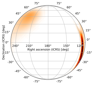
../_images/jup_plotting-examples_52_2.png

but, by default, the image will be rotated. Fortunately, the final rot tuple (corresponding to FITS LONPOLE) simply rotates about the central reference axis, and the image can be oriented right-side-up by setting it to 180 (the default LONPOLE value HPMOC uses for zenithal projections):

[27]:

m.plot(height=720, width=720, projection='SIN', rot=(60, -15, 180))

[27]:

<astropy.visualization.wcsaxes.core.WCSAxes at 0x127ee2d50>

/Users/s/anaconda3/envs/hpmoc-dev/lib/python3.7/site-packages/astropy/visualization/wcsaxes/grid_paths.py:73: RuntimeWarning: invalid value encountered in greater
  discontinuous = step[1:] > DISCONT_FACTOR * step[:-1]
/Users/s/anaconda3/envs/hpmoc-dev/lib/python3.7/site-packages/astropy/visualization/wcsaxes/grid_paths.py:73: RuntimeWarning: invalid value encountered in greater
  discontinuous = step[1:] > DISCONT_FACTOR * step[:-1]
/Users/s/anaconda3/envs/hpmoc-dev/lib/python3.7/site-packages/astropy/visualization/wcsaxes/grid_paths.py:73: RuntimeWarning: invalid value encountered in greater
  discontinuous = step[1:] > DISCONT_FACTOR * step[:-1]
/Users/s/anaconda3/envs/hpmoc-dev/lib/python3.7/site-packages/astropy/visualization/wcsaxes/grid_paths.py:73: RuntimeWarning: invalid value encountered in greater
  discontinuous = step[1:] > DISCONT_FACTOR * step[:-1]

../_images/jup_plotting-examples_54_2.png

Again, 2-angle rotations do this automatically; we can therefore make this same plot with

[28]:

m.plot(height=720, width=720, projection='SIN', rot=(60, -15))

[28]:

<astropy.visualization.wcsaxes.core.WCSAxes at 0x128182450>

/Users/s/anaconda3/envs/hpmoc-dev/lib/python3.7/site-packages/astropy/visualization/wcsaxes/grid_paths.py:73: RuntimeWarning: invalid value encountered in greater
  discontinuous = step[1:] > DISCONT_FACTOR * step[:-1]
/Users/s/anaconda3/envs/hpmoc-dev/lib/python3.7/site-packages/astropy/visualization/wcsaxes/grid_paths.py:73: RuntimeWarning: invalid value encountered in greater
  discontinuous = step[1:] > DISCONT_FACTOR * step[:-1]
/Users/s/anaconda3/envs/hpmoc-dev/lib/python3.7/site-packages/astropy/visualization/wcsaxes/grid_paths.py:73: RuntimeWarning: invalid value encountered in greater
  discontinuous = step[1:] > DISCONT_FACTOR * step[:-1]
/Users/s/anaconda3/envs/hpmoc-dev/lib/python3.7/site-packages/astropy/visualization/wcsaxes/grid_paths.py:73: RuntimeWarning: invalid value encountered in greater
  discontinuous = step[1:] > DISCONT_FACTOR * step[:-1]

../_images/jup_plotting-examples_56_2.png

Zoomed Plots

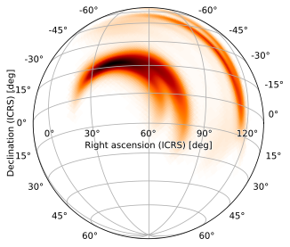
It’s possible to zoom in on an area of interest by modifying the hdelta and vdelta parameters, which override the angular widths of the reference pixels. If we’re zooming in on an area of interest, however, we’d be better served using a zenithal projection, e.g. the gnomonic projection (equivalent to that used by healpy.gnomview). We can choose a different projection from one of those specified in `hpmoc.plot <../hpmoc.plot.rst#hpmoc.plot.plot>`__, specifying it by name (or one of its aliases), saving us the trouble of setting up a custom world coordinate system (astropy.wcs.WCS) instance. A gnomonic plot, centered at the default location with default pixel sizes (hdelta and vdelta automatically calculated), looks like this:

[29]:

m.plot(projection='TAN', rot=(60, -15))

[29]:

<astropy.visualization.wcsaxes.core.WCSAxes at 0x1206138d0>

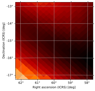
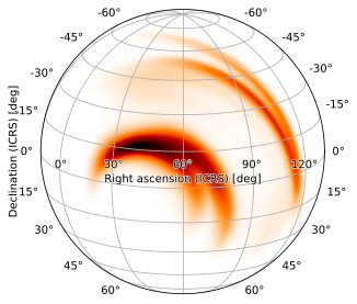
../_images/jup_plotting-examples_58_1.png

At this zoom level, we can clearly see the individual HEALPix pixels, but it’s hard to see the larger structure of the central probability region. We can zoom out by tweaking vdelta and hdelta, which in practice is easiest to do by trial and error until your plot looks how you’d like it to:

[30]:

m.plot(projection='TAN', vdelta=0.3, hdelta=0.3, rot=(60, -15))

[30]:

<astropy.visualization.wcsaxes.core.WCSAxes at 0x128a7b910>

../_images/jup_plotting-examples_60_1.png

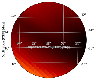
Fixed Angular Width

You can also figure out exactly what hdelta and vdelta mean by, again, referencing Calabretta and Greisen (2002) and looking up the relevant projection’s interpretation of CDELT1 and CDELT (the width and height, respectively, of the reference pixel in a given projection, which, it should be noted, does not correspond to the angular width of that pixel in most cases).

This is usually not worth the trouble, but can sometimes be useful, particularly when automating plotting, though in this case the problem can sometimes most easily be solved by choosing an appropriate projection; for example, if you want a circular window of radius 5 degrees, you can easily plot it using the zenithal equidistant projection:

[31]:

from hpmoc.plot import ARC_CDELT_BASE

radius_deg = 5
delta = ARC_CDELT_BASE * min(radius_deg, 180) / 180
m.plot(projection='ARC', hdelta=delta, vdelta=delta,
       rot=(60, -15), frame_class='elliptical')

[31]:

<astropy.visualization.wcsaxes.core.WCSAxes at 0x12840b890>

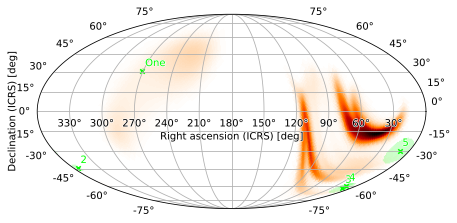
../_images/jup_plotting-examples_62_1.png

Scatterplots

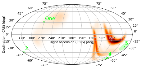
You can plot point sources, including their error regions, by passing collections of points (as hpmoc.points.PointsTuple instances) to plot. You can specify each point source using its right ascension, declination (both in degrees), (optional) error region size (in degrees), and (optional) label, i.e. the name of that source (unnamed sources will be labeled with their index within the PointsTuple):

[32]:

from hpmoc.points import PointsTuple, Rgba

pts1 = PointsTuple(
    [
        (271., 31., 2., 'One'),
        (355., -44., 3.),
        (15., -62., 5.),
        (16., -60., 3.),
        (10., -30., 10.),
    ]
)

m.plot(pts1)

[32]:

<astropy.visualization.wcsaxes.core.WCSAxes at 0x128dc1150>

../_images/jup_plotting-examples_64_1.png

The font is a little small for the point source labels; we can fix this by passing keyword arguments for WCSAxes.text as the scatter_labels argument:

[33]:

m.plot(pts1, scatter_labels={'fontsize': 16})

[33]:

<astropy.visualization.wcsaxes.core.WCSAxes at 0x1287d2410>

../_images/jup_plotting-examples_66_1.png

We can also increase the DPI of the figure to increase legibility:

[34]:

m.plot(pts1, fig={'dpi': 100})

[34]:

<astropy.visualization.wcsaxes.core.WCSAxes at 0x128bf8450>

../_images/jup_plotting-examples_68_1.png

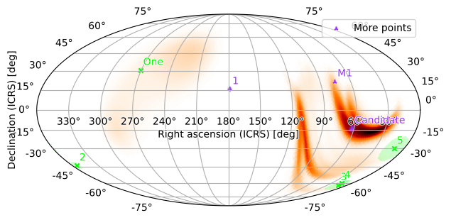
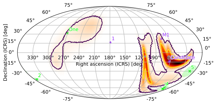
You can plot multiple sets of points, which can be distinguished by color, marker, and legend label (M1 location from here):

[35]:

from astropy.units import Unit

pts2 = PointsTuple(
    points=[
        (179., 16., 2.),
        (62, -14, 3., 'Candidate'),
        (
            (5*Unit('hourangle')+34.5*Unit('arcmin')).to('deg').value,
            (22*Unit('deg')+1*Unit('arcmin')).to('deg').value,
            (6*Unit('arcmin')).to('deg').value,
            'M1'
        )
    ],
    rgba=Rgba(0.6, 0.2, 1, 0.5),
    marker='2',
    label='More points',
)
m.plot(pts1, pts2, fig={'dpi': 100})
plt.legend()

[35]:

<matplotlib.legend.Legend at 0x128d38c10>

../_images/jup_plotting-examples_70_1.png

You can also bundle point sources with a related skymap by appending them to the point_sources field of a PartialUniqSkymap:

[36]:

m.point_sources = [pts1, pts2]
m.plot(fig={'dpi': 100})
plt.legend()

[36]:

<matplotlib.legend.Legend at 0x127a88e50>

../_images/jup_plotting-examples_72_1.png

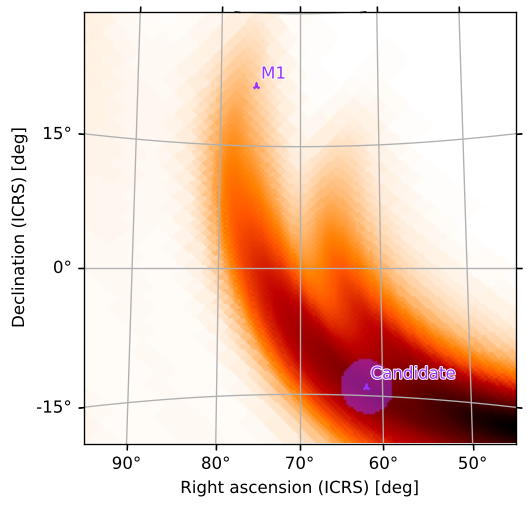
Again, we can rotate and zoom in on a region of interest; our point sources will now be plotted automatically (since they are contained in the point_sources field):

[37]:

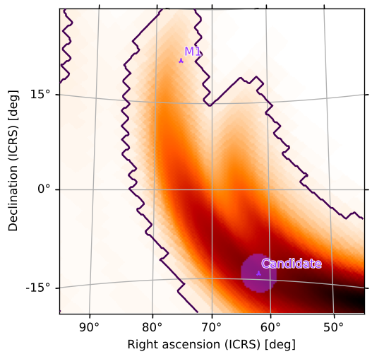
m.plot(fig={'dpi': 120}, rot=(70, 5), vdelta=0.3, hdelta=0.3, projection='TAN')

[37]:

<astropy.visualization.wcsaxes.core.WCSAxes at 0x127e21290>

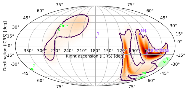
../_images/jup_plotting-examples_74_1.png

Contours around Credible Regions

We can also add contours around credible/containment regions of the plot. For example, to get the smallest region containing 90% of the GW probability, run

[38]:

m.plot(fig={'dpi': 100}, cr=[.9])

[38]:

<astropy.visualization.wcsaxes.core.WCSAxes at 0x1299a9350>

../_images/jup_plotting-examples_76_1.png

Or, with our zoomed plot:

[39]:

m.plot(fig={'dpi': 120}, rot=(70, 5), vdelta=0.3, hdelta=0.3, projection='TAN', cr=[0.9])

[39]:

<astropy.visualization.wcsaxes.core.WCSAxes at 0x129ec0cd0>

../_images/jup_plotting-examples_78_1.png

We can easily add the 50% contour as well:

[40]:

m.plot(fig={'dpi': 120}, cr=[0.5, 0.9])

[40]:

<astropy.visualization.wcsaxes.core.WCSAxes at 0x12a204fd0>

../_images/jup_plotting-examples_80_1.png

[41]:

m.plot(fig={'dpi': 120}, rot=(70, 5), vdelta=0.3, hdelta=0.3, projection='TAN', cr=[0.5, 0.9])

[41]:

<astropy.visualization.wcsaxes.core.WCSAxes at 0x12a9fc890>

../_images/jup_plotting-examples_81_1.png

Our example “Candidate” event is clearly within both contours.

Multi-layered plots

Sometimes it is desirable to overlay several images. For example, we can visualize both the skymap itself and the size of its pixels by plotting them as a semi-transparent overlay using the alpha keyword and the same axis as the original skymap. We can include colorbars for both and pick colormaps which are visually distinguishable. We also tweak the figure size and cbar keyword arguments to improve the layout of the final result:

[42]:

ax = m.plot(fig={'figsize': (6, 5)}, cbar={'pad': 0.05}, cmap='bone_r')
m.orders(as_skymap=True).plot(ax=ax, alpha=0.15, cmap='rainbow', cbar={'pad': 0.1})
ax.set_title('S200105ae')

[42]:

Text(0.5, 1.0, 'S200105ae')

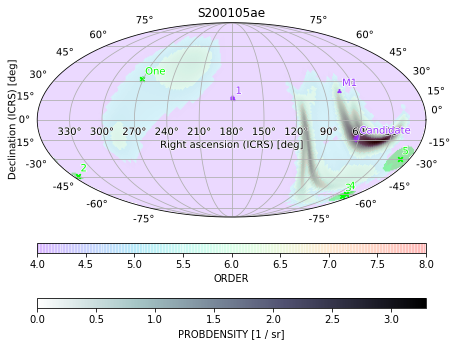
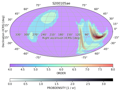
../_images/jup_plotting-examples_83_1.png

We can also get rid of the point sources again, since they are visually distracting, and increase the opacity of the pixel sizes (ORDER) to emphasize that layer:

[43]:

m.point_sources = []
ax = m.plot(fig={'figsize': (6, 5)}, cbar={'pad': 0.05}, cmap='bone_r')
m.orders(as_skymap=True).plot(ax=ax, alpha=0.4, cmap='rainbow', cbar={'pad': 0.1})
ax.set_title('S200105ae')

[43]:

Text(0.5, 1.0, 'S200105ae')

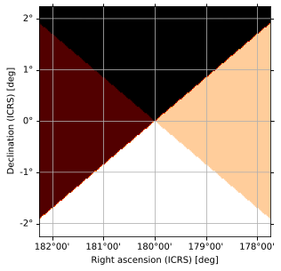
../_images/jup_plotting-examples_85_1.png

If we wanted to emphasize the pixel size completely, we could plot it alone and then simply plot some contours from the original skymap over it. We can entirely hide an image (but not the contours or associated point sources) by setting cmap=None and label and color our contours with the cr_format and cr_kwargs arguments:

[44]:

ax = m.orders(as_skymap=True).plot(projection='CAR', fig={'dpi': 120}, cbar=True)
m.plot(ax=ax, cmap=None, cr=[0.5, 0.9, 0.99],
       cr_format=lambda l, _: f"{l*100:2.0f}% CR",
       cr_kwargs={'colors': ['aquamarine', 'teal', 'blue']})

[44]:

<astropy.visualization.wcsaxes.core.WCSAxes at 0x12d1f5750>

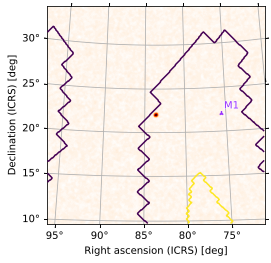
../_images/jup_plotting-examples_87_1.png

You can, of course, use this approach to layer skymaps over images from arbitrary FITS sources. Let’s plot a random Swift-BAT high-SNR FITS image (downloaded from astroquery) alongside our second set of point sources with only the credible region boundaries from our skymap showing:

[45]:

from astropy.wcs import WCS
from astroquery.skyview import SkyView

# get a Swift-BAT high-SNR FITS image from around M1 (Crab Nebula)
hdu = SkyView.get_images(position='M1', survey='BAT SNR 150-195')[0][0]
ax = plt.subplot(1, 1, 1, projection=WCS(hdu.header))
ax.imshow(hdu.data, cmap='gist_heat_r')
m.plot(pts2, ax=ax, cmap=None, cr=[0.5, 0.9])

[45]:

<matplotlib.axes._subplots.WCSAxesSubplot at 0x12e8ab910>

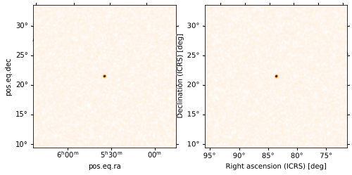
../_images/jup_plotting-examples_89_1.png

We can also interpolate a standard FITS image (as long as the astropy.wcs.WCS coordinate transforms are implemented in FITS) using HPMOC. This lets us put images in arbitrary projections into the same pixelization, making it easy to plot them on the arbitrary axes, do analyses with them, etc. You can see that the results are indistinguishable from the original:

[46]:

# interpolate the FITS image
mh = PartialUniqSkymap(hdu.data, WCS(hdu.header))

# plot a comparison
fig = plt.figure(figsize=(8, 4))
axw = fig.add_subplot(1, 2, 1, projection=WCS(hdu.header))
axw.imshow(hdu.data, cmap='gist_heat_r')
axh = mh.plot(fig=axw.figure, subplot=(1, 2, 2), projection=WCS(hdu.header))
axh.grid(False)

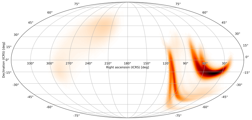
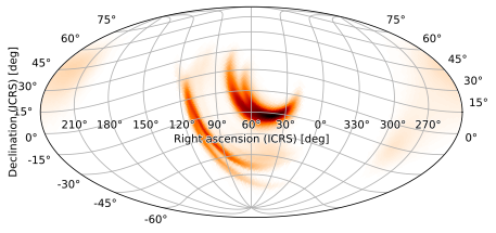
../_images/jup_plotting-examples_91_0.png

More usefully, we can do an all-sky plot of an arbitrarily-projected FITS image with almost no effort. We can label the missing regions as gray and increase the resolution of the image to capture the small bright region in the center:

[47]:

mh.plot(missing_color='gray', width=1000, height=500)

[47]:

<astropy.visualization.wcsaxes.core.WCSAxes at 0x12eb00710>

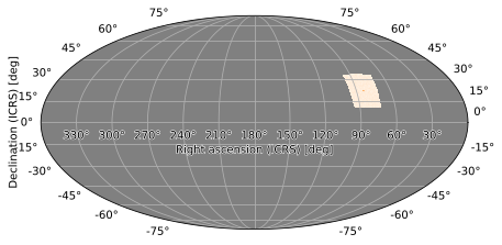
../_images/jup_plotting-examples_93_1.png

Note that by default, nearest neighbor interpolation will be used (at around 5-10 times the resolution of the original image), and units (and particularly area calculations/conversions) will not be handled automatically.

Subplots

You can plot to subplots using the subplot argument. For example, we can manually make a grid of subplots using plt.subplot and pass the corresponding axes to plot. We can accomplish the same thing by passing the subplot argument to plot:

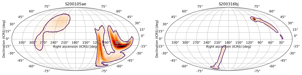
[48]:

m2 = PartialUniqSkymap.read(BAYESTAR_NEST_FITS_GZ_1024, strategy='ligo')
ax1 = m.plot(fig={'figsize': (16, 4)}, subplot=(1, 2, 1), cr=[0.9])
ax1.set_title('S200105ae')
ax2 = m2.plot(fig=ax1.figure, subplot=(1, 2, 2), cr=[0.9])
ax2.set_title('S200316bj')

[48]:

Text(0.5, 1.0, 'S200316bj')

../_images/jup_plotting-examples_96_1.png

This also works with matplotlib.gridspec.SubplotSpec as the subplot argument (if you want to plot to a specific axes on a matplotlib.gridspec.GridSpec). We can also get the axis manually with matplotlib.figure.Figure.add_subplot and pass it as the ax argument.

Grid Plots

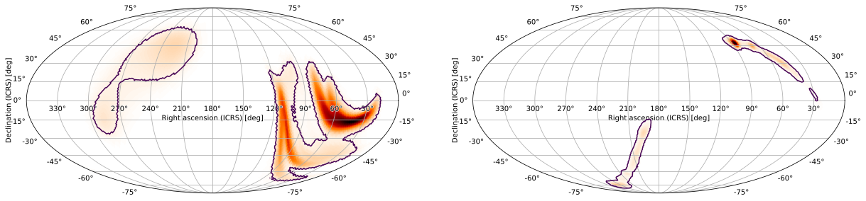
It is often useful to compare skymaps, or look at the same skymap with different sets of point sources, plot settings, or projections. The quickest way to do this using HPMOC is to use hpmoc.plot.gridplot, which uses GridSpec behind the scenes. We can quickly do the same as above:

[49]:

m.gridplot(m2, cr=[0.9])

[49]:

(GridSpec(1, 2, width_ratios=[2.0, 2.0]),
 [[<matplotlib.axes._subplots.WCSAxesSubplot at 0x12f67f4d0>,
   <matplotlib.axes._subplots.WCSAxesSubplot at 0x12f68c1d0>]])

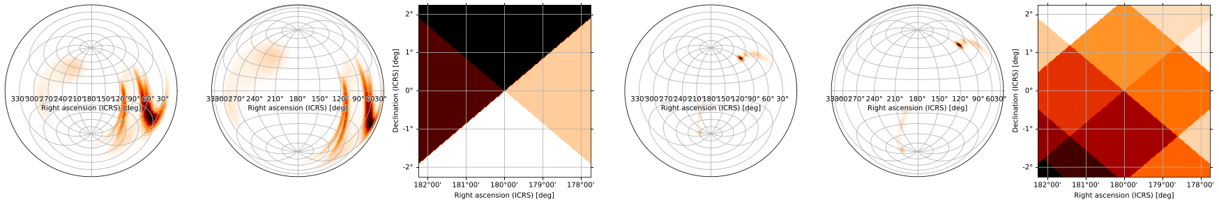
../_images/jup_plotting-examples_98_1.png

You can also specify multiple projections for each skymap:

[50]:

m.gridplot(m2, projections=['ARC', 'ZEA', 'TAN'])

[50]:

(GridSpec(1, 6, width_ratios=[1.0, 1.0, 1.0, 1.0, 1.0, 1.0]),
 [[<matplotlib.axes._subplots.WCSAxesSubplot at 0x12f8fe810>,
   <matplotlib.axes._subplots.WCSAxesSubplot at 0x12f641e10>],
  [<matplotlib.axes._subplots.WCSAxesSubplot at 0x12f388e50>,
   <matplotlib.axes._subplots.WCSAxesSubplot at 0x12f254610>],
  [<matplotlib.axes._subplots.WCSAxesSubplot at 0x12ff35390>,
   <matplotlib.axes._subplots.WCSAxesSubplot at 0x12f25a890>]])

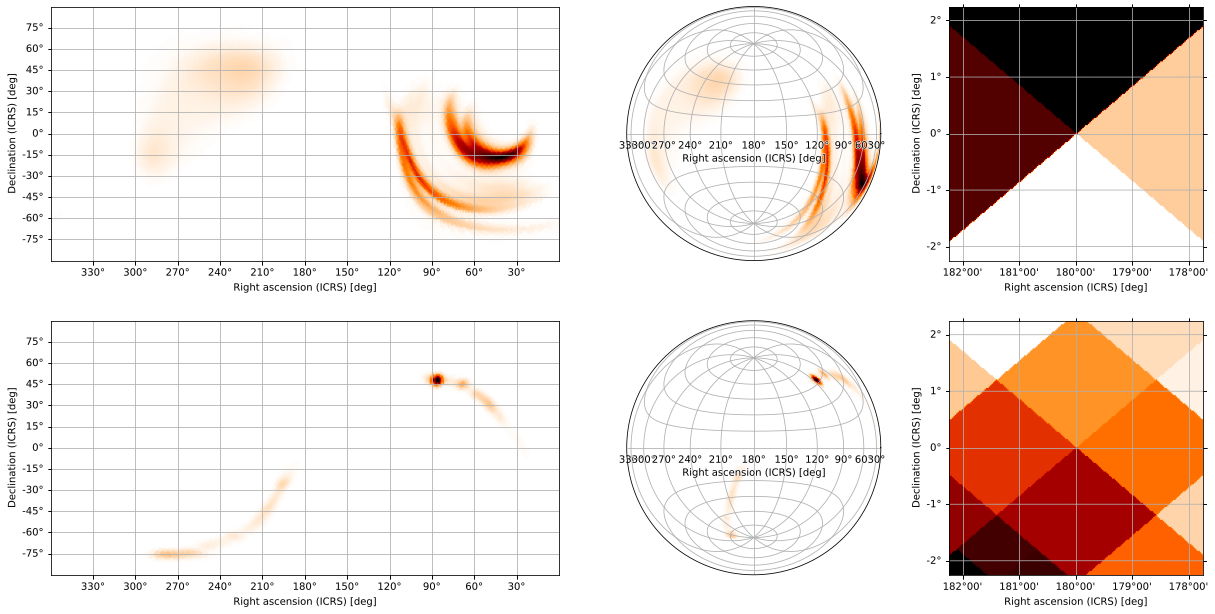
../_images/jup_plotting-examples_100_1.png

Specify how many columns (where different projections of the same skymap are grouped into a single column) appear on each row:

[51]:

m.gridplot(m2, projections=['CAR', 'ZEA', 'TAN'], ncols=1)

[51]:

(GridSpec(2, 3, width_ratios=[2.0, 1.0, 1.0]),
 [[<matplotlib.axes._subplots.WCSAxesSubplot at 0x130811810>,
   <matplotlib.axes._subplots.WCSAxesSubplot at 0x12f67fd90>],
  [<matplotlib.axes._subplots.WCSAxesSubplot at 0x1308119d0>,
   <matplotlib.axes._subplots.WCSAxesSubplot at 0x130777710>],
  [<matplotlib.axes._subplots.WCSAxesSubplot at 0x130f10490>,
   <matplotlib.axes._subplots.WCSAxesSubplot at 0x12d58c7d0>]])

../_images/jup_plotting-examples_102_1.png

The first return value is the GridSpec used to arrange the subplots, while the second is a list whose rows correspond to each projection in the projections argument and are themselves lists of axes corresponding to each skymap. In other words, gridplot(...)[1][p][s] is the axes containing a plot of the s $^\text{th}$ skymap using the p $^\text{th}$ projection. You can use this to modify specific subplots, add titles to all plots, etc:

[52]:

maps = [m, *[PartialUniqSkymap.read(f, strategy='ligo') for f in
                        (BAYESTAR_NEST_FITS_GZ_1024, CWB_NEST_FITS_GZ_128,
                         CWB_RING_FITS_GZ_128)]]
gs, axs = gridplot(*maps, projections=['CEA', 'TAN'])
for *axx, title in zip(*axs, ('S200105ae', 'S200316bj-1-Preliminary',
                              'S200114f-3-Initial', 'S200129m-3-Initial')):
    for ax in axx:
        ax.set_title(title)

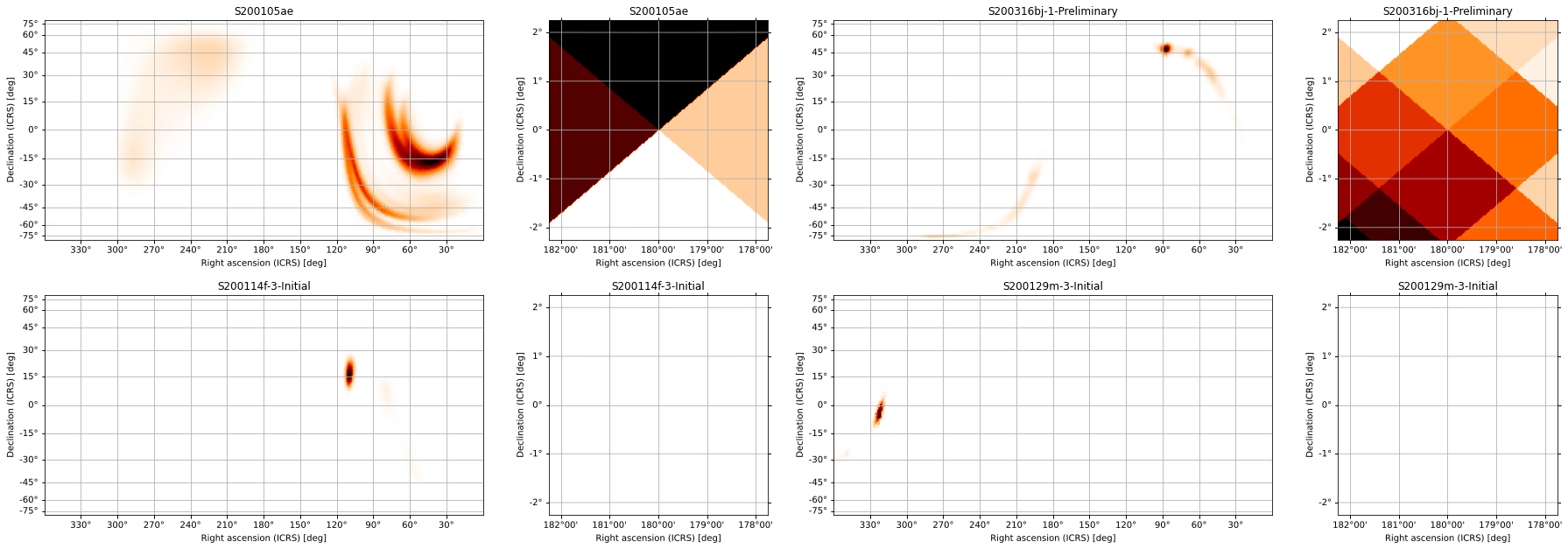
../_images/jup_plotting-examples_104_0.png

We can add scatter plots of points of interest using the scatters argument to pass a list of PointsTuple instances for each skymap, and we can pass separate keyword arguments to hpmoc.plot.plot for each subplot (following the same shape as the returned axes). We can use this, for example, to adjust the zoom level and rotation of the gnomonic projections separately from the all-sky views and to set the vmax values for the color maps consistently across projections. Arguments shared across all subplots can be passed as keyword arguments to gridplot, as we will do for vmin=0:

[53]:

maps = [m, *[PartialUniqSkymap.read(f, strategy='ligo') for f in
                        (BAYESTAR_NEST_FITS_GZ_1024, CWB_NEST_FITS_GZ_128,
                         CWB_RING_FITS_GZ_128)]]
gs, axs = gridplot(*maps, scatters=[[pts2]]*4, projections=['CEA', 'TAN'],
         subplot_kwargs=[[{'vmax': s.max().value} for s in maps],
                         [{'vdelta': 0.4, 'hdelta': 0.4,
                           'rot': (70, 5), 'vmax': s.max().value}
                          for s in maps]], vmin=0, ncols=1, cr=[0.9])
for *axx, title in zip(*axs, ('S200105ae', 'S200316bj-1-Preliminary',
                              'S200114f-3-Initial', 'S200129m-3-Initial')):
    for ax in axx:
        ax.set_title(title)

/Users/s/anaconda3/envs/hpmoc-dev/lib/python3.7/site-packages/astropy/visualization/wcsaxes/core.py:234: UserWarning: No contour levels were found within the data range.
  cset = super().contour(*args, **kwargs)

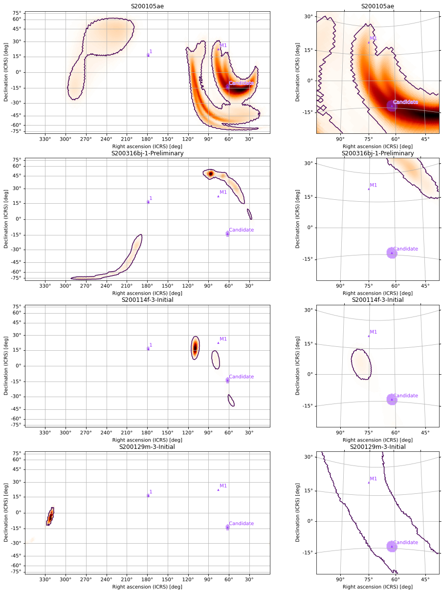
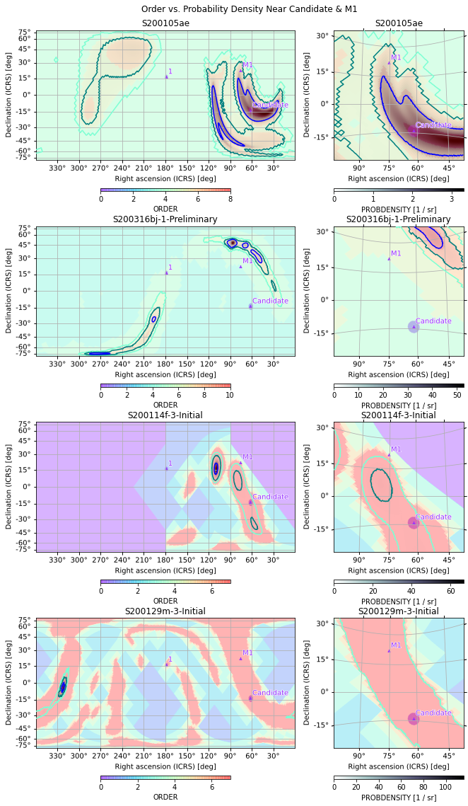
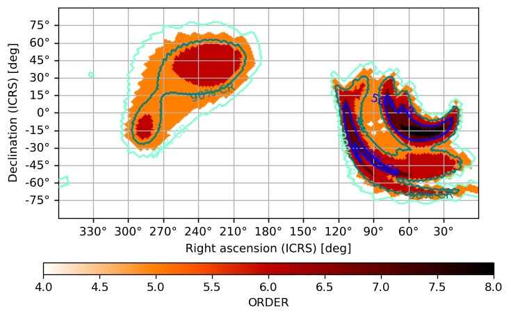
../_images/jup_plotting-examples_106_1.png

We can add colorbars and layer our images as we were able to do with plot, though this time instead of passing ax to our second invocation of the plotting function, we pass the returned GridSpec and axes list (after tweaking some of the spacing arguments to make the layout look better). We can use this approach to make quite intricate visualizations for multiple skymaps with fairly little effort:

[54]:

maps = [m, *[PartialUniqSkymap.read(f, strategy='ligo') for f in
                        (BAYESTAR_NEST_FITS_GZ_1024, CWB_NEST_FITS_GZ_128,
                         CWB_RING_FITS_GZ_128)]]
gs, axs = gridplot(*maps, wspace=0.2, hspace=0.05, wshrink=0.7,
                   scatters=[[pts2]]*4, ncols=1, top=0.95,
                   projections=['CEA', 'TAN'], height=360,
                   subplot_kwargs=[[{'width': 720, 'vmax': s.max().value}
                                    for s in maps],
                                   [{'width': 360, 'vdelta': 0.2,
                                     'hdelta': 0.2, 'cbar': True,
                                     'rot': (70, 5), 'vmax': s.max().value}
                                    for s in maps]],
                   cr=[0.5, 0.9, 0.99], vmin=0., cmap='bone_r',
                   cr_kwargs={'colors': ['aquamarine', 'teal', 'blue']})
for *axx, title in zip(*axs, ('S200105ae', 'S200316bj-1-Preliminary',
                              'S200114f-3-Initial', 'S200129m-3-Initial')):
    for ax in axx:
        ax.set_title(title)
orders = [s.orders(as_skymap=True) for s in maps]
gridplot(*orders, projections=axs, fig=gs, alpha=0.3,
         cmap='rainbow', vmin=0,
         subplot_kwargs=[[{'cbar': {'shrink': 0.5}, 'vmax': o.max()}
                          for o in orders], [{'cmap': None}]*4])
plt.suptitle("Order vs. Probability Density Near Candidate & M1")

/Users/s/anaconda3/envs/hpmoc-dev/lib/python3.7/site-packages/astropy/visualization/wcsaxes/core.py:234: UserWarning: No contour levels were found within the data range.
  cset = super().contour(*args, **kwargs)
/Users/s/anaconda3/envs/hpmoc-dev/lib/python3.7/site-packages/hpmoc/plot.py:886: MatplotlibDeprecationWarning: Adding an axes using the same arguments as a previous axes currently reuses the earlier instance.  In a future version, a new instance will always be created and returned.  Meanwhile, this warning can be suppressed, and the future behavior ensured, by passing a unique label to each axes instance.
  frame_class=frame_class)

[54]:

Text(0.5, 0.98, 'Order vs. Probability Density Near Candidate & M1')

../_images/jup_plotting-examples_108_2.png